Distributions

Truncated normal

multiple-inference’s truncated normal distribution allows for concave truncation sets.

import matplotlib.pyplot as plt
import numpy as np
import seaborn as sns
from scipy.stats import norm, truncnorm as scipy_truncnorm

from multiple_inference.stats import truncnorm, quantile_unbiased

sns.set()
x = np.linspace(-1, 2)
sns.lineplot(x=x, y=truncnorm([(-1, 0), (1, 2)]).cdf(x))
plt.show()

Quantile unbiased distribution

The quantile-unbiased distribution is the distribution of an unknown mean of a normal distribution given

1. A realized value of the distribution,

2. A truncation set in which the realized value had to fall, and

3. A known variance

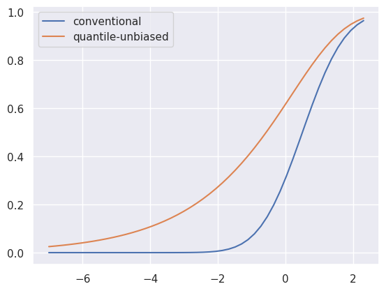
In the example below, the realized value is .5, the truncation set is \([0, \infty)\), and the variance (scale) is 1 by default. The interpretation of the CDF plot is, “there is a \(CDF(x)\) chance that the mean of the normal distribution from which the realized value (.5) was drawn is less than \(x\)”.

We compare the quantile-unbiased distribution to a normal distribution centered on the realized value.

dist = quantile_unbiased(.5, truncation_set=[(0, np.inf)])
x = np.linspace(dist.ppf(.025), dist.ppf(.975))
sns.lineplot(x=x, y=norm.cdf(x, .5), label="conventional")
sns.lineplot(x=x, y=dist.cdf(x), label="quantile-unbiased")
plt.show()

q = .5
f"There is a {q} chance that the mean of the normal distribution from which the realized value was drawn is less than {dist.ppf(q)}"

'There is a 0.5 chance that the mean of the normal distribution from which the realized value was drawn is less than -0.5725351048077288'