Multiple Inference Cookbook

This template is an 80-20 solution for multiple inference. It uses many of the latest techniques in multiple inference to answer the following questions:

1. Compare to zero. Which parameters are significantly different from zero?

2. Compare to the average. Which parameters are significantly different from the average (i.e., the average value across all parameters)?

3. Pairwise comparisons. Which parameters are significantly different from which other parameters?

4. Distribution. What does the distribution of parameters look like?

5. Ranking. What is the ranking of each parameter?

6. Selection. Which parameters might be the largest (i.e., the highest ranked)?

7. Inference after ranking. What are the values of the parameters given their rank? e.g., What is the value of the parameter with the largest estimated value?

Click the badge below to use this template on your own data. This will open the notebook in a Jupyter binder.

Instructions:

1. Upload a file named data.csv to this folder with your conventional estimates. Open data.csv to see an example. In this file, we named our dependent variable “dep_variable”, and have estimated parameters named “policy0”,…, “policy9”. The first column of data.csv contains the conventional estimates \(m\) of the unknown parameters. The remaining columns contain consistent estimates of the covariance matrix \(\Sigma\). In data.csv, \(m=(0, 1,..., 9)\) and \(\Sigma = I\).

2. Modify the code if necessary.

3. Run the notebook.

Runtime warnings and long running times

If you are estimating many parameters or the parameters effects are close together, you may see RuntimeWarning messages and experience long runtimes. Runtime warnings are common, usually benign, and can be safely ignored.

import matplotlib.pyplot as plt
import numpy as np
import seaborn as sns

from multiple_inference.bayes import Improper, Nonparametric, Normal
from multiple_inference.confidence_set import ConfidenceSet, AverageComparison, PairwiseComparison, SimultaneousRanking
from multiple_inference.rank_condition import RankCondition

data_file = "data.csv"
alpha = .05

np.random.seed(0)
sns.set()

First, we’ll summarize and plot your original (conventional) estimates.

model = Improper.from_csv(data_file, sort=True)
results = model.fit(title="Conventional estimates")
results.summary(alpha=alpha)

Conventional estimates

	coef	pvalue (1-sided)	[0.025	0.975]
policy9	9.000	0.000	7.040	10.960
policy8	8.000	0.000	6.040	9.960
policy7	7.000	0.000	5.040	8.960
policy6	6.000	0.000	4.040	7.960
policy5	5.000	0.000	3.040	6.960
policy4	4.000	0.000	2.040	5.960
policy3	3.000	0.001	1.040	4.960
policy2	2.000	0.023	0.040	3.960
policy1	1.000	0.159	-0.960	2.960
policy0	0.000	0.500	-1.960	1.960

Dep. Variable	y

results.point_plot(alpha=alpha)
plt.show()

Next, we’ll create a reconstruction plot. A reconstruction plot shows what we would expect the conventional estimates to look like if your estimates were correct.

For example, imagine we ran a randomized control trial in which we tested the effects of ten treatments. We then obtained our conventional estimates using OLS and rank ordered them. Now, suppose our conventional estimates are correct (i.e., assume the true effect of each treatment follows its OLS distribution). What would our new estimates look like if we reran the experiment, estimated the treatment effects by OLS, and rank ordered them again?

Ideally, the new conventional estimates would look like our original conventional estimates. Below, the blue dots show the simulated distribution of new estimates. The orange x’s show our original conventional estimates. So, ideally, the blue dots should be on top of the orange x’s.

Conventional estimates are more spread out than the true parameters in expectation. That is, conventional estimates often suggest that some parameters are very different from others, even if they are all similar. We call this problem fictitious variation. Our conventional estimates suffer from fictitious variation when the blue dots are more spread out than the orange x’s.

results.reconstruction_point_plot(title="Conventional estimates reconstruction plot")
plt.show()

Compare to zero

First, we’ll test which parameters significantly differ from zero. There are at least two criteria we could apply in answering this question. First, we might want to control the false discovery rate. The false discovery rate is the proportion of rejected hypotheses that are truly null. This testing procedure begins by converting p-values into q-values. We start by splitting the distribution of p-values into two components: a uniform distribution and a right-skewed distribution. (If a null hypothesis is true, its p-value will follow a uniform distribution. If a null hypothesis is false, its p-value will follow a right-skewed distribution.) Using these components, we can estimate the proportion of true nulls we would reject (the q-value) by rejecting all hypotheses with a p-value below a given significance threshold. Look at the “qvalue” column in the table below. Suppose we reject all null hypotheses with a q-value below 0.05. In that case, about 5% of the rejected hypotheses are truly null.

Second, we might want to control the family-wise error rate. The family-wise error rate is the probability of making at least one false discovery. That is, it is the probability of rejecting at least true null hypothesis. We can control the family-wise error rate using simultaneous confidence intervals. Suppose we estimated \(K\) parameters. Simultaneous confidence intervals begin by forming a \(K\)-dimensional rectangle such that all the parameters fall within this rectangle with 95% probability. Then, they “project” this \(K\)-dimensional rectangle onto the dimension for a specific parameter to obtain that parameter’s simultaneous confidence interval. By construction, all the parameters fall within their simultaneous confidence interval with 95% probability. Look at the “pvalue” column in the table below. Suppose we reject all null hypotheses with a p-value below 0.05. In that case, there is a 5% chance that any rejected hypotheses are truly null. Simultaneous confidence intervals are similar to a Bonferroni correction but have higher power.

model = ConfidenceSet.from_csv(data_file, sort=True)
results = model.fit()
results.summary(alpha=alpha)

Confidence set results

	coef (conventional)	pvalue	qvalue	0.95 CI lower	0.95 CI upper
policy9	9.000	0.000	0.000	6.190	11.810
policy8	8.000	0.000	0.000	5.190	10.810
policy7	7.000	0.000	0.000	4.190	9.810
policy6	6.000	0.000	0.000	3.190	8.810
policy5	5.000	0.000	0.000	2.190	7.810
policy4	4.000	0.001	0.000	1.190	6.810
policy3	3.000	0.028	0.001	0.190	5.810
policy2	2.000	0.371	0.018	-0.810	4.810
policy1	1.000	0.979	0.114	-1.810	3.810
policy0	0.000	1.000	0.323	-2.810	2.810

Dep. Variable	y

ax = results.point_plot(alpha=alpha)
ax.axvline(0, linestyle="--")
plt.show()

We can also use a stepdown improvement to increase power while controlling the family-wise error rate. This is analogous to Holm’s stepdown improvement on the Bonferroni correction.

results.test_hypotheses(alpha=alpha)

	param>0	param<0
policy9	True	False
policy8	True	False
policy7	True	False
policy6	True	False
policy5	True	False
policy4	True	False
policy3	True	False
policy2	False	False
policy1	False	False
policy0	False	False

Compare to the average

Next, we’ll use q-values and simultaneous confidence intervals to discover which parameters significantly differ from the average (i.e., the average across all parameters). This is similar to what we did before. However, instead of constructing q-values and simultaneous confidence intervals for the parameters \(\mu_k\), we’ll construct them for the difference between the parameters and the average \(\mu_k - \mathbf{E}[\mu_j]\).

model = AverageComparison.from_csv(data_file, sort=True)
results = model.fit()
results.summary(alpha=alpha)

Confidence set results

	coef (conventional)	pvalue	qvalue	0.95 CI lower	0.95 CI upper
policy9	4.500	0.000	0.000	1.835	7.165
policy8	3.500	0.002	0.000	0.835	6.165
policy7	2.500	0.081	0.004	-0.165	5.165
policy6	1.500	0.677	0.039	-1.165	4.165
policy5	0.500	1.000	0.164	-2.165	3.165
policy4	-0.500	1.000	0.164	-3.165	2.165
policy3	-1.500	0.677	0.039	-4.165	1.165
policy2	-2.500	0.081	0.004	-5.165	0.165
policy1	-3.500	0.002	0.000	-6.165	-0.835
policy0	-4.500	0.000	0.000	-7.165	-1.835

Dep. Variable	y

The x-axis in the plot below is the estimated difference between each parameter and the average \(\mu_k - \mathbf{E}[\mu_j]\).

ax = results.point_plot(alpha=alpha)
ax.axvline(0, linestyle="--")
plt.show()

results.test_hypotheses(alpha=alpha)

	param>0	param<0
policy9	True	False
policy8	True	False
policy7	False	False
policy6	False	False
policy5	False	False
policy4	False	False
policy3	False	False
policy2	False	False
policy1	False	True
policy0	False	True

Pairwise comparisons

Next, we’ll use q-values and simultaneous confidence intervals to perform pairwise comparisons. Instead of constructing q-values and simultaneous confidence intervals for the individual parameters \(\mu_k\), we’ll construct them for all pairwise differences \(\mu_j - \mu_k \quad \forall j, k\).

First, we’ll perform hypothesis testing using q-values by setting criterion="fdr" for “false discovery rate.” Green squares in the heatmap below indicate that we have rejected the null hypothesis \(H_{j,k}: \mu_k = \mu_j\), where \(j\) is the parameter on the x-axis and \(k\) is the parameter on the y-axis. Red squares indicate that we have not rejected the null hypothesis. Of the rejected hypotheses, we expect that at most \(\alpha\) proportion are truly null.

model = PairwiseComparison.from_csv(data_file, sort=True)
results = model.fit()
results.hypothesis_heatmap(alpha=alpha, triangular=True, criterion="fdr")
plt.show()

Second, we’ll perform hypothesis testing using simultaneous confidence intervals by setting criterion="fwer" for “family-wise error rate.” Green squares in the heatmap below indicate that we have rejected the null hypothesis \(H_{j,k}: \mu_j \leq \mu_k\). That is, we have concluded that the parameter on the x-axis is greater than the parameter on the y-axis. Red squares indicate that we have not rejected the null hypothesis. We expect that we have rejected at least one truly will hypothesis with probability \(\alpha\).

results.hypothesis_heatmap(alpha=alpha, triangular=True, criterion="fwer")
plt.show()

Distributions

Next, we’ll use Bayesian estimators to understand the distribution of parameters. Bayesian estimators begin with a prior distribution and then update that belief based on data using Bayes’ Theorem to obtain a posterior distribution.

Classical Bayesian estimators take the prior as given. However, we can often obtain better estimates by using empirical Bayes to estimate the prior from the data. For example, imagine predicting MLB players’ on-base percentage (OBP) next season. We might predict that a player’s OBP next season will be the same as his OBP in the previous season. But how can we predict the OBP for a rookie with no batting history? One solution is to predict that the rookie’s OBP will be similar to last season’s rookies’ OBP. In Bayesian terms, we’ve constructed a prior belief about next season’s rookies’ OBP using data from the previous season’s rookies’ rookies’ OBP.

Empirical Bayes uses the same logic. Imagine randomly selecting one parameter \(\mu_k\) and putting the data we used to estimate it in a locked box. We can use the data about the remaining parameters to estimate a prior distribution for \(\mu_k\).

Empirical Bayes estimators can be parametric or non-parametric. Parametric empirical Bayes assumes the shape of the prior distribution. Nonparametric empirical Bayes does not assume the shape of the prior distribution. Below, we apply a parametric empirical Bayes estimator assuming a normal prior distribution.

First, let’s plot one parameter’s prior, conventional, and posterior distributions.

model = Normal.from_csv(data_file, sort=True)
parametric_results = model.fit()
parametric_results.line_plot(0)
plt.show()

Next, let’s create a reconstruction plot for the Bayesian estimator. This plot shows what we would expect the conventional estimates to look like if the Bayesian model were correct. Remember that we want the blue dots to be on top of the orange x’s.

Compare the reconstruction plot for the Bayesian estimates (below) to the reconstruction plot for the conventional estimates near the top of the notebook. Looking at the reconstruction plot for the conventional estimates at the top of the notebook, you’ll likely see that the conventional estimates are too spread out (the blue dots are more spread out than the orange x’s). Looking at the reconstruction plot for the Bayesian estimates below, you’ll likely see that the Bayesian estimates are appropriately spread out (the blue dots are on top of the orange x’s).

parametric_results.reconstruction_point_plot(title="Parametric empirical Bayes reconstruction plot")
plt.show()

If the reconstruction plot looks good, does that mean our parametric assumption (that the prior is a normal distribution) is correct? What if the assumption is wrong?

Amazingly, parametric empirical Bayes estimators usually give us more accurate point estimates than conventional estimators regardless of the prior distribution. Some, like the James-Stein estimator, are mathematically guaranteed to do so. Additionally, we can estimate “robust” confidence intervals that have correct coverage regardless of the prior distribution.

Let’s summarize and plot the Bayesian estimates using robust confidence intervals.

parametric_results.summary(alpha=alpha, robust=True)

Bayesian estimates

	coef	pvalue (1-sided)	[0.025	0.975]
policy9	8.455	0.000	6.495	10.414
policy8	7.576	0.000	5.617	9.535
policy7	6.697	0.000	4.738	8.656
policy6	5.818	0.000	3.859	7.777
policy5	4.939	0.000	2.980	6.899
policy4	4.061	0.000	2.101	6.020
policy3	3.182	0.000	1.223	5.141
policy2	2.303	0.007	0.344	4.262
policy1	1.424	0.066	-0.535	3.383
policy0	0.545	0.282	-1.414	2.505

Dep. Variable	y

parametric_results.point_plot(alpha=alpha, robust=True)
plt.show()

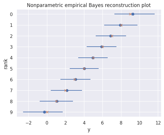
Let’s repeat this exercise with a nonparametric empirical Bayes estimator. Remember, parametric empirical Bayes estimators assume the shape of the prior distribution (e.g., normal). Nonparametric empirical Bayes estimators do not assume the shape of the prior distribution. We’ll start by plotting the prior, conventional estimate, and posterior for a single parameter.

model = Nonparametric.from_csv(data_file, sort=True)
nonparametric_results = model.fit()
nonparametric_results.line_plot(0)
plt.show()

nonparametric_results.reconstruction_point_plot(title="Nonparametric empirical Bayes reconstruction plot")
plt.show()

/home/docs/checkouts/readthedocs.org/user_builds/dsbowen-conditional-inference/envs/latest/lib/python3.10/site-packages/multiple_inference-1.2.0-py3.10.egg/multiple_inference/bayes/base.py:67: UserWarning: Model does not provide a joint posterior distribution. I'll assume the marginal posterior distributions are independent. Rank estimates and likelihood and Wasserstein approximations may be unreliable.

nonparametric_results.summary(alpha=alpha)

Bayesian estimates

	coef	pvalue (1-sided)	[0.025	0.975]
policy9	8.774	0.000	6.848	10.725
policy8	7.802	0.000	5.864	9.740
policy7	6.834	0.000	4.900	8.756
policy6	5.874	0.000	3.998	7.792
policy5	4.949	0.000	3.095	6.848
policy4	4.051	0.000	2.152	5.905
policy3	3.126	0.001	1.208	5.002
policy2	2.166	0.014	0.244	4.100
policy1	1.198	0.113	-0.740	3.136
policy0	0.226	0.411	-1.725	2.152

Dep. Variable	y

nonparametric_results.point_plot(alpha=alpha)
plt.show()

Should you use a parametric or nonparametric empirical Bayes estimator? In my experience, parametric empirical Bayes is better for a small number of parameters, and nonparametric empirical Bayes is better for a large number of parameters. If both estimators give similar point estimates, trust the one with wider confidence intervals (usually the parametric version). If the estimators give very different point estimates, my rule of thumb is to trust parametric empirical Bayes when estimating fewer than 50 parameters and nonparametric empirical Bayes otherwise.

This notebook is an 80-20 solution for multiple inference. For a 90-50 solution, use cross-validation to decide between parametric and nonparametric empirical Bayes.

Ranking

Next, we’ll estimate each parameter’s rank. For example, we might say that we’re 95% confident that the parameter with the largest estimated value is genuinely one of the largest three parameters. One way to do this is by sampling from a Bayesian estimator’s posterior distribution and seeing how often parameter \(k\) falls in a certain rank.

parametric_results.rank_point_plot(alpha=alpha)
plt.show()

nonparametric_results.rank_point_plot(alpha=alpha)
plt.show()

Selection

Selection is closely related to ranking. We often want to select a set of parameters that we’re confident rank near the top.

For example, we often want to know parameters might be the largest (i.e., highest-ranked). That is, we want a set of parameters containing the best (largest) parameter with 95% confidence. We can use Bayesian estimators to construct this set. Starting from an empty set, we continue adding parameters until we’re confident that one of them is genuinely the best according to the posterior distribution.

Parameters with “True” next to them in the table below are in this set. Parameters with “False” next to them are not.

parametric_results.compute_best_params(alpha=alpha, criterion="fwer")

policy9     True
policy8     True
policy7     True
policy6    False
policy5    False
policy4    False
policy3    False
policy2    False
policy1    False
policy0    False
dtype: bool

nonparametric_results.compute_best_params(alpha=alpha, criterion="fwer")

policy9     True
policy8     True
policy7     True
policy6    False
policy5    False
policy4    False
policy3    False
policy2    False
policy1    False
policy0    False
dtype: bool

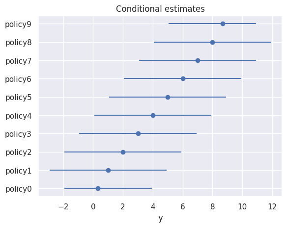
Inference after ranking

Finally, we’ll estimate parameters given the rank of their conventional estimates. For example, imagine we ran a randomized control trial testing ten treatments and want to estimate the effectiveness of the top-performing treatment.

One property we want our estimators to have is quantile-unbiasedness. An estimator is quantile-unbiased if the true parameter falls below its \(\alpha\)-quantile estimate with probability \(\alpha\) given its estimated rank. For example, the true effect of the top-performing treatment should fall below its median estimate half the time.

Similarly, we want confidence intervals to have correct conditional coverage. Correct conditional coverage means that the parameter should fall within our \(\alpha\)-level confidence interval with probability \(1-\alpha\) given its estimated rank. For example, the true effect of the top-performing treatment should fall within its 95% confidence interval 95% of the time.

Below, we compute the optimal quantile-unbiased estimates and conditionally correct confidence intervals for each parameter given its rank.

model = RankCondition.from_csv(data_file, sort=True)
results = model.fit(title="Conditional estimates")
results.summary(alpha=alpha)

/home/docs/checkouts/readthedocs.org/user_builds/dsbowen-conditional-inference/envs/latest/lib/python3.10/site-packages/multiple_inference-1.2.0-py3.10.egg/multiple_inference/stats.py:468: RuntimeWarning: divide by zero encountered in log
/home/docs/checkouts/readthedocs.org/user_builds/dsbowen-conditional-inference/envs/latest/lib/python3.10/site-packages/multiple_inference-1.2.0-py3.10.egg/multiple_inference/stats.py:476: RuntimeWarning: divide by zero encountered in scalar divide
/home/docs/checkouts/readthedocs.org/user_builds/dsbowen-conditional-inference/envs/latest/lib/python3.10/site-packages/scipy/optimize/_numdiff.py:576: RuntimeWarning: invalid value encountered in subtract
  df = fun(x) - f0

Conditional estimates

	coef (median)	pvalue (1-sided)	[0.025	0.975]
policy9	8.686	0.000	5.067	10.933
policy8	8.000	0.001	4.078	11.922
policy7	7.000	0.001	3.078	10.922
policy6	6.000	0.003	2.078	9.922
policy5	5.000	0.009	1.078	8.922
policy4	4.000	0.023	0.078	7.922
policy3	3.000	0.058	-0.922	6.922
policy2	2.000	0.136	-1.922	5.922
policy1	1.000	0.285	-2.922	4.922
policy0	0.314	0.406	-1.933	3.933

Dep. Variable	y

results.point_plot(alpha=alpha)
plt.show()

Conditional inference is a strict requirement. Conditionally quantile-unbiased estimates can be highly variable. And conditionally correct confidence intervals can be unrealistically long. We can often obtain more reasonable estimates by focusing on unconditional inference instead of conditional inference.

Imagine we ran our randomized control trial 10,000 times and want to estimate the effect of the top-performing treatment. We need conditional inference if we’re interested the subset of trials where a specific parameter \(k\) was the top performer. However, we can use unconditional inference if we’re only interested in being right “on average” across all 10,000 trials.

Below, we use hybrid estimates to compute approximately quantile-unbiased estimates and unconditionally correct confidence intervals for each parameter.

If you don’t know whether you need conditional or unconditional inference, use unconditional inference.

results = model.fit(beta=.005, title="Hybrid estimates")
results.summary(alpha=alpha)

Hybrid estimates

	coef (median)	pvalue (1-sided)	[0.025	0.975]
policy9	8.687	0.005	5.680	10.977
policy8	8.000	0.005	4.680	11.320
policy7	7.000	0.005	3.680	10.320
policy6	6.000	0.005	2.680	9.320
policy5	5.000	0.005	1.680	8.320
policy4	4.000	0.005	0.680	7.320
policy3	3.000	0.055	-0.320	6.320
policy2	2.000	0.140	-1.320	5.320
policy1	1.000	0.288	-2.320	4.320
policy0	0.313	0.409	-1.977	3.320

Dep. Variable	y

results.point_plot(alpha=alpha)
plt.show()

Both Bayesian and rank condition estimators give parameter estimates and confidence intervals. Which ones should we use?

We should use Bayesian estimators if our goal is to understand the distribution of parameters. If, however, our goal is to estimate a parameter given its rank (e.g., the top-performing parameter), the answer is less clear. In my experience, Bayesian point estimates are better than rank condition point estimates, but rank condition confidence intervals are better than Bayesian confidence intervals. For example, if you want to estimate the top-performing parameter, I recommend writing your discussion section using the Bayesian point estimate and the rank condition (hybrid) confidence interval.

Again, this template is an 80-20 solution for multiple inference. For a 90-50 solution, use cross-validation to decide whether Bayesian or rank condition estimates are better for your data set.