Distributions

Truncated normal

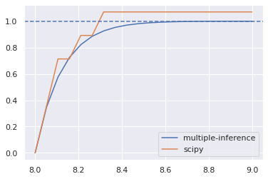
multiple-inference’s truncated normal distribution has two advantages over scipy’s. First, it uses the state-of-the-art exponential tilting method which improves performance in the tails. Second, it allows for concave truncation sets.

In the example below, we plot the cumulative distribution function (CDF) of a standard normal truncated to the interval \((8, \infty)\). As we can see, scipy’s CDF evaluated at 9 is greater than 1. Clearly, this cannot be correct, because a CDF cannot exceed 1 by definition. By contrast, multiple inference’s truncated normal CDF does not exceed 1.

import matplotlib.pyplot as plt
import numpy as np
import seaborn as sns
from scipy.stats import norm, truncnorm as scipy_truncnorm

from multiple_inference.stats import truncnorm, quantile_unbiased

sns.set()
x = np.linspace(8, 9, num=20)
ax = sns.lineplot(x=x, y=truncnorm([(8, np.inf)]).cdf(x), label="multiple-inference")
sns.lineplot(x=x, y=scipy_truncnorm(8, np.inf).cdf(x), label="scipy")
ax.axhline(1, linestyle="--")
plt.show()

/home/docs/checkouts/readthedocs.org/user_builds/dsbowen-conditional-inference/envs/stable/lib/python3.8/site-packages/multiple_inference-1.1.0-py3.8.egg/multiple_inference/stats.py:562: RuntimeWarning: divide by zero encountered in log
/home/docs/checkouts/readthedocs.org/user_builds/dsbowen-conditional-inference/envs/stable/lib/python3.8/site-packages/multiple_inference-1.1.0-py3.8.egg/multiple_inference/stats.py:570: RuntimeWarning: divide by zero encountered in double_scalars
/home/docs/checkouts/readthedocs.org/user_builds/dsbowen-conditional-inference/envs/stable/lib/python3.8/site-packages/scipy/optimize/_numdiff.py:576: RuntimeWarning: invalid value encountered in subtract
  df = fun(x) - f0

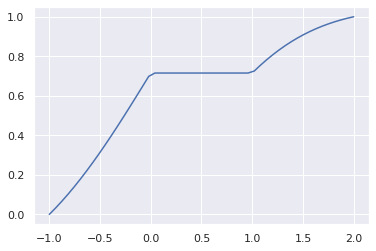
Now, let’s plot the CDF of a standard normal truncated to the interval \((-1, 0) \cup (1, 2)\).

x = np.linspace(-1, 2)
sns.lineplot(x=x, y=truncnorm([(-1, 0), (1, 2)]).cdf(x))
plt.show()

Quantile unbiased distribution

The quantile-unbiased distribution is the distribution of an unknown mean of a normal distribution given

1. A realized value of the distribution,

2. A truncation set in which the realized value had to fall, and

3. A known variance

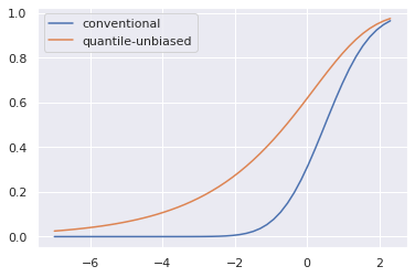
In the example below, the realized value is .5, the truncation set is \([0, \infty)\), and the variance (scale) is 1 by default. The interpretation of the CDF plot is, “there is a \(CDF(x)\) chance that the mean of the normal distribution from which the realized value (.5) was drawn is less than \(x\)”.

We compare the quantile-unbiased distribution to a normal distribution centered on the realized value.

dist = quantile_unbiased(.5, truncation_set=[(0, np.inf)])
x = np.linspace(dist.ppf(.025), dist.ppf(.975))
sns.lineplot(x=x, y=norm.cdf(x, .5), label="conventional")
sns.lineplot(x=x, y=dist.cdf(x), label="quantile-unbiased")
plt.show()

q = .5
f"There is a {q} chance that the mean of the normal distribution from which the realized value was drawn is less than {dist.ppf(q)}"

'There is a 0.5 chance that the mean of the normal distribution from which the realized value was drawn is less than -0.5725351048077288'